Conway's Gradient of Life

Tuesday, May 5, 2020 · 3 min read

And now, a magic trick. Before you is a 239-by-200 Conway’s Game of Life board:

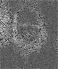
What happens if we start from this configuration and take a single step of the game? Here is a snapshot of the next generation:

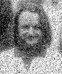
Amazing! It’s a portrait of John Conway! (Squint!)

How does this trick work? (It’s not a hoax — you can try it yourself at copy.sh/life using this RLE file.)

Well, let’s start with how it doesn’t work. Reversing Life configurations exactly — the art of “atavising” — is a hard search problem, and doing it at this scale would be computationally infeasible. Imagine searching through $ 2^{239\times200} $ possible configurations! Surely that is hopeless… indeed, the talk I linked shares some clever algorithms that nonetheless take a full 10 minutes to find a predecessor for a tiny 10-by-10 board.

But it turns out that approximately reversing a Life configuration is much easier — instead of a tricky discrete search problem, we have an easy continuous optimization problem for which we can use our favorite algorithm, gradient descent.

Here is the idea: Start with a random board configuration $ b $ and compute $ b^\prime $, the result after one step of Life. Now, for some target image $ t $ compute the derivative $ \frac{\partial}{\partial b} \sum|b^\prime-t| $, which tells us how to change $ b $ to make $ b^\prime $ closer to $ t $. Then take a step of gradient descent, and rinse and repeat!

Okay, okay, I know what you’re thinking: Life isn’t differentiable! You’re right. Life is played on a grid of bools, and there is no way the map $ b \mapsto b^\prime $ is continuous, let alone differentiable.

But suppose we could make a “best effort” differentiable analogue? Let us play Life on a grid of real numbers that are 0 for “dead” cells and 1 for “live” cells. Can we “implement” a step of Life using only differentiable operations? Let’s try.

We will look at each cell $ c $ individually. The first step is to count our live neighbors. Well, if “live” cells are 1 and “dead” cells are 0, then we can simply add up the values of all 8 of our neighbors to get our live neighbor count $ n $. Indeed, if we wanted to be clever, we could implement this efficiently as a convolution with this kernel:

\[ \begin{bmatrix} 1 & 1 & 1 \\ 1 & 0 & 1 \\ 1 & 1 & 1 \end{bmatrix} \]

Good, so we know $ n $ and of course our own 0/1 value $ c $. The next step is to figure out whether this cell will be alive in the next generation. Here are the rules:

1. If the cell is alive, $ c = 1 $, then it stays alive if and only if $ n = 2 $ or $ n = 3 $.
2. If the cell is dead, $ c = 0 $, then it comes to life if and only if $ n = 3 $.

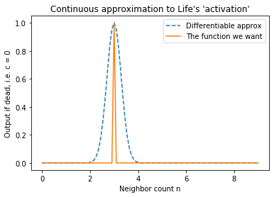
Let us approach (2) first. What function is 1 when $ n = 3 $ and 0 otherwise? The “spike-at-3” function, of course. That’s not differentiable, but a narrow Gaussian centered at 3 is almost the same thing! If scaled appropriately, the Gaussian is one at input 3, and almost zero everywhere else. See this graph:

Similarly, for (1) an appropriately-scaled Gaussian centered at 2.5 gets the job done. Finally, we can mux these two cases under gate $ c $ by simple linear interpolation. Because $ c \approx 0 $ or $ c \approx 1 $, we know that $ ca + (1-c)b $ is just like writing if c then a else b.

That’s it! We now have a differentiable function, which looks like this:

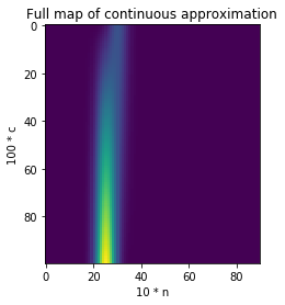
Note that it’s worth “clamping” the output of that function to 0 or 1 using, say, the tanh function. That way cell values always end up close to 0 or 1.

Okay, great! Now all that’s left to do is to write this in PyTorch and call .backward()…

…and it begins to learn, within seconds! Here is a GIF of $ b $ at every 100 steps of gradient descent.

(Note: This GIF is where the target image $ t $ is an all-white rectangle; my janky PyTorch gradient descent finds sparse configurations that give birth to an “overpopulated” field where nearly 90% of cells are alive.)

Looking at that GIF, the beautiful labyrinthine patterns reminded me of something seemingly unrelated: the skin of a giant pufferfish. Here’s a picture from Wikipedia:

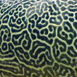
And here’s a zoomed-in 100-by-100 section of the finished product from above:

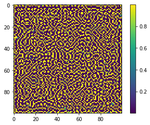
Patterns like the one on the pufferfish come about as a result of “symmetry-breaking,” when small perturbations disturb an unstable homogeneous state. The ideas were first described by Alan Turing (and thus the patterns are called Turing Patterns). Here’s his 1952 paper.

I can’t help but wonder if there’s a reaction-diffusion-model-esque effect at work here as well, the symmetry being broken by the random initialization of $ b $. If that’s the case, it would create quite a wonderful connection between cells, cellular automata, Turing-completeness, and Turing patterns…

(Curious? Here is the Python program I used to play these games. Enjoy!)